Getting started

The gdf repository directory comes with a main.py driver Python file and a init_gdf_default.py initialization file. It is expected that the user would only need to change (normally, just a few) of the parameters in the initialization file to obtain the distributions and associated moments in a desired time interval.

A example GDF reconstruction

To get started with your first reconstruction using the gdf repository, run the following in your terminal from the repository directory. Make sure you have activated your environment where you have installed gdf.

python main.py init_gdf_default

This should generate a few diagnostic figures, plots of reconstruction and super-resolution under the Figures/ directory, as well as a pkl file under the Outputs/ directory. Two of these generated figures that we would like to highlight at the outset are

• Fig. 1 which shows a comparison between the SPAN-Ai grids in field aligned coordinates (FAC) and the corresponding reconstructed distribution at the same grid points from the polar-cap Slepian reconstruction. These are plotted using matplotlib.pyplot.tricontourf since the data is on an irregular grid. This figure can be found in Figures/span_rec_contour/.

• Fig. 2 which shows the final reconstructed GDF after being super-resolved on a fine Cartesian grid. This figure can be found in Figures/super_res/. All subsequent moments are computed using super-resolved distributions and not the crude SPAN-Ai FAC distributions.

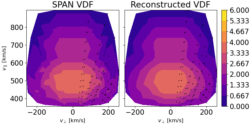
Fig. 1 Left: A matplotlib.pyplot.tricontourf representation of the SPAN-Ai VDF after rotating the grids into field aligned coordinates (FAC). Right: Same, but for the polar cap reconstructed GDF evaluated at the FAC grid locations. The colorbar is obtained from normalizing the log-scaled distributions.

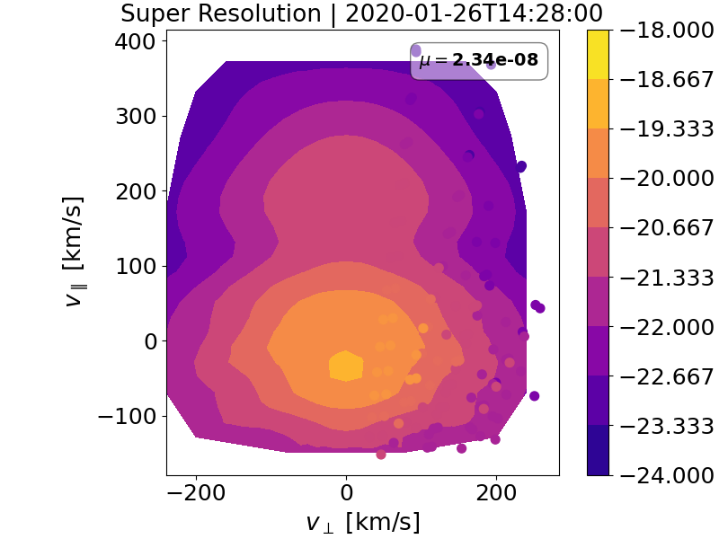
Fig. 2 Final super-resolved image from the Slepians-on-a-polar-cap basis reconstruction. The background colormap is obtained from a matplotlib.pyplot.tricontourf of the high-resolution Cartesian super-resolved grid. The overplotted colored grids denote the SPAN-Ai measurements for visual comparison to assess goodness-of-fit. The colorbar is in log-scale but in original VDF units.

Understanding the initialization file

# init_gdf_default.py
# This is a template for primary initization file.
# 'global': parameters needed for any method of reconstruction
# 'polcap', 'cartesian', 'hybrid' are parameters specific to particular methods of reconstruction

config = {
    'global': {
        'METHOD'          : 'hybrid',
        'TRANGE'          : ['2020-01-26T14:28:00', '2020-01-26T20:30:59'],   # Define the time range to load in from pyspedas
        'CLIP'            : True,
        'START_INDEX'     : 0,
        'NSTEPS'          : 10,                                               # use None for entire TRANGE interval
        'CREDS_PATH'      : None,                                             # path to the <.json> file containing credentials
        'COUNT_THRESHOLD' : 2,
        'SAVE_FIGS'       : True,
        'SAVE_PKL'        : True,
        'MIN_METHOD'      : 'L-BFGS-B',
        'NPTS_SUPER'      : 49,
        'MCMC'            : False,
        'MCMC_WALKERS'    : 6,
        'MCMC_STEPS'      : 200,
    },
    'polcap': {
        'TH'              : 30,
        'LMAX'            : 12,
        'N2D_POLCAP'      : None,
        'P'               : 3,
        'SPLINE_MINCOUNT' : 7,
    },
    'cartesian': {
        'N2D_CART'        : 16,
    },
    'hybrid': {
        'LAMBDA'          : 1e-1,
    }
}

The initialization file is supposed to be the primary interface for a standard user. While there are a number of listed parameters, TRANGE, START_INDEX and NTEPS are the three primary parameters which we think the user would interact with the most. Descriptions for all the parameters are provided in the table below.

Table 1 Description of parameters in the init_gdf_default.py initialization file.

Parameter	Type	Description
TRANGE	list of str	Start and end times in ISO 8601 standard format in UTC YYYY-MM-DD-Thh:mm:ss
CLIP	bool	Whether to clip to specified TRANGE or keep entire day’s data.
START_INDEX	int	Index of first desired time stamp for gdf with respect to the start time in TRANGE.
NSTEPS	int or None	Number of timestamps to analyze starting at START_INDEX. Use None for entire TRANGE.
CREDS_PATH	str or None	Path to a json file containing credentials to access SWEAP and FIELDS proprietary data.
COUNT_THRESHOLD	int	Particle count threshold below which grid points are ignored from reconstructions.
SAVE_FIGS	bool	Flag if the final (and diagnostic) figures should be saved under directories in Figures/.
SAVE_PKL	bool	Flag if the final metadata should be stored as a pkl file in the Outputs/ directory.
MIN_METHOD	str	Minimization method used in the scipy.optimize.minimize. Optimal choice is ‘L-BFGS-B’.
NPTS_SUPER	int or tuple of ints	Number of super-resolved points in a uniform Cartesian grid of (\(v_{\perp},\, v_{\parallel}\)). This can be a tuple if (NPTSx, NPTSy) where \(x\) is along \(v_{\perp}\) and \(y\) is along \(v_{\parallel}\).
MCMC	bool	Flag to use a MCMC refinement of the gyroaxis, provides error esimtates on the gyro-centroid.
MCMC_WALKERS	int	Number of MCMC walkers to be used. Need to use 3 minimum walkers.
MCMC_STEPS	int	Number of MCMC steps for each walker. Optimal choice: (6 MCMC_WALKERS, 200 MCMC_STEPS).
TH	float	Polar cap extent in degrees about the magnetic field axis used for generating Slepians.
LMAX	int	Maximum angular degree for constructing the 1D Slepian basis on a polar cap..
N2D_POLCAP	int or None	The number of polar-cap Slepian functions to be used for reconstructions.
P	int (default: 3)	The degree of the B-spline used for discretizing in velocity phase space.
SPLINE_MINCOUNT	int	Minimum number of grid points to be contained in each B-spline shell.
N2D_CART	int	The Shannon number for the Cartesian Slepian basis.
LAMBDA	float	The imposed similarity in the cost function term \(\lambda \left(G_1 \, m_1 - G_2 \, m_2 \right)^2\).